A PLC (Programmable Logic Controller) is an industrial computer used for automation of electromechanical processes, such as control of machinery on factory assembly lines, amusement rides, or light fixtures. PLCs are expected to work flawlessly for years in industrial environments that are hazardous to the very microelectronic components that give modern PLCs their excellent flexibility and precision.
Prior to PLCs, many of these control tasks were solved with contactor or relay controls. This is often referred to as hardwired control. Circuit diagrams had to be designed, electrical components specified and installed, and wiring lists created. Electricians would then wire the components necessary to perform a specific task. If an error was made the wires had to be reconnected correctly. A change in function or system expansion required extensive component changes and rewiring.
Objectives
This article aims to:
1- Learn the basics of ladder logic programming.
2- Familiarize the students with SIMATIC S7 software to program Siemens S7-400 PLC.
3- Implement different logic functions using PLC.
4- Understand the function of each Siemens S7-400 PLC modules.
Theory
Before you start using PLC, it is convenient to know and understand its architecture. See figure 1.
As shown in figure 1, PLC consists of the following parts:
1) POWER SUPPLY: Provides the voltage needed to run the primary PLC components.
2) I/O MODULES: Provides signal conversion and isolation between the internal logic-level signals inside the PLC and the field’s high level signal.
3) PROCESSOR SYSTEM: Provides intelligence to command and govern the activities of the entire PLC systems.
4) PROGRAMMING DEVICE: Used to enter the desired program that will determine the sequence of operation.
Figure 1: PLC architecture
The following are some advantages of PLC over other microcontrollers:
1) Cost effective for controlling complex systems.
2) Flexible and can be reapplied to control other systems.
3) Computational abilities allow more sophisticated control.
4) Trouble shooting aids making programming easier and reduce downtime.
5) Small physical size, so shorter project time.
In this experiment Siemens S7-400 PLC will be used, table 1 presents the main components of this model.
Table 1: Siemens S7-400 PLC main components
You can notice from figure 2 that the common of the digital input module is connected to the ground of the circuit while the common of the digital output module is connected to the power source.
Figure 2: Simple Connection using Siemens S7-400 PLC
The last figure shows a switch connected to the input I0.0 in the digital input module,and an LED connected to the output Q0.0 in the output module.
Ladder Logic Programming
Figure 3 shows electrical continuity, when SW1 is closed, the current will flow from L-1 to L-2 and energize the load.
Even though PLC ladder logic was modeled after the conventional relay ladder, there is no electrical continuity in PLC ladder logic. PLC ladder rungs should have logical continuity in order for the output to be energized. PLC ladder program uses familiar terms like “rungs”, “normally open” and “normally closed” contacts, as illustrated in table 2.
Table 2: Fundamental contacts and coils instructions of PLC ladder logic programming
In a ladder logic program, there is no physical conductor that carries the input signal through to the output. Each rung in the ladder diagram is a program statement. This program statement consists of a condition or sometimes conditions, along with some type of action.
Inputs are the conditions, and the action, or output, is the result of the conditions. As in case of physical wiring hardware devices connected in series or parallel, PLC also combines ladder program instructions in series or parallel. However, rather than working in series or parallel, the PLC combines instructions logically using logic operators like: AND, OR, and NOT. These operators are used to combine the instructions on a PLC rung to make the outcome of each rung either true or false.
1. AND-logic function:
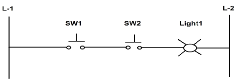
A series circuit of two switches can be regarded as AND logic function. In figure 4, both switches (SW1 AND SW2) must be closed to have electrical continuity to energize the output (Light-1). Hence the keyword here is AND.
Figure 4: AND-logic function
The circuit shown in figure 5 represents a schematic ladder logic rung for the circuit shown in figure 4. When switch 1 and switch 2 are closed the output coil will be energized.
Figure 5: Ladder logic diagram for AND function
2. OR-logic function:
A parallel circuit of two switches can be regarded as OR logic function. In figure 6, one of the switches (SW1 OR SW2) must be closed to have electrical continuity to energize the output (Light-1). Hence the keyword here is OR.
Figure 6: OR-logic function
The circuit shown in figure 7 represents a schematic ladder logic rung for the circuit shown in figure 6. If switch 1 or switch 2 is closed the output coil will be energized.
Figure 7: Ladder logic diagram for OR function
3. The PARALLEL NOT logic function:
Figure 8 shows ladder diagram for the parallel NOT logic function and its truth table is illustrated in table 3.
Figure 8: Ladder logic diagram for parallel NOT function
Table 3: Parallel NOT logic function truth table
Set Coil Instruction
Figure 9 shows the symbol of set coil instruction:
Figure 9: The symbol of set coil instruction
Description: ---( S )--- (Set Coil) is executed only if the RLO of the preceding instructions is "1" (power flows to the coil). If the RLO is "1" the specified <address> of the element is set to "1". An RLO = 0 has no effect and the current state of the element’s specified address remains unchanged.
The following example illustrates the operation of set coil instruction, see figure 10:
Figure 10: Set coil instruction example
The signal state of output Q4.0 is "1" if one of the following conditions exists:
• The signal state is "1" at inputs I0.0 and I0.1
• Or the signal state is "0" at input I0.2.
If the RLO is "0", the signal state of output Q4.0 remains unchanged.
Reset Coil Instruction
Figure 11 shows the symbol of reset coil instruction:
Figure 11: The symbol of reset coil instruction
Description: ---( R )--- (Reset Coil) is executed only if the RLO of the preceding instructions is "1" (power flows to the coil). If power flows to the coil (RLO is "1"), the specified <address> of the element is reset to "0". A RLO of "0" (no power flow to the coil) has no effect and the state of the element’s specified address remains unchanged. The <address> may also be a timer (T no.) whose timer value is reset to "0" or a counter (C no.) whose counter value is reset to "0".
The following example illustrates the operation of reset instruction, see figure 12:
Figure 12: Reset coil instruction example
The signal state of output Q4.0 is reset to "0" if one of the following conditions exists:
• The signal state is "1" at inputs I0.0 and I0.1
• Or the signal state is "0" at input I0.2.
If the RLO is "0", the signal state of output Q4.0 remains unchanged.
The signal state of timer T1 is only reset if:
• the signal state is "1" at input I0.3.
The signal state of counter C1 is only reset if:
• the signal state is "1" at input I0.4..
• Positive RLO Edge Detection
• Figure 13 shows the symbol of Positive RLO Edge Detection instruction.
Figure 13: Positive RLO Edge Detection Symbol
Description: ---( P )--- (Positive RLO Edge Detection) detects a signal change in the address from "0" to "1" and displays it as RLO = "1" after the instruction. The current signal state in the RLO is compared with the signal state of the address, the edge memory bit. If the signal state of the address is "0" and the RLO was "1" before the instruction, the RLO will be "1" (pulse) after this instruction, and "0" in all other cases. The RLO prior to the instruction is stored in the address.
Table 4 illustrates the function of each parameter of Positive RLO Edge Detection:
Table 4: Positive RLO edge detection parameters
The following example illustrates the operation of Positive RLO Edge Detection, see figure 14:
Figure 14: Positive RLO Edge Detection Example
• The edge memory bit M0.0 saves the old RLO state. When there is a signal change at the RLO from "0" to "1", the program jumps to label CAS1.
• Negative RLO Edge Detection
• Figure 15 shows the symbol of Negative RLO Edge Detection instruction.
Figure 15: Negative RLO Edge Detection Symbol
Description: ---( N )--- (Negative RLO Edge Detection) detects a signal change in the address from "1" to "0" and displays it as RLO = "1" after the instruction. The current signal state in the RLO is compared with the signal state of the address, the edge memory bit. If the signal state of the address is "1" and the RLO was "0" before the instruction, the RLO will be "1" (pulse) after this instruction, and "0" in all other cases. The RLO prior to the instruction is stored in the address.
Table 3 illustrates the function of each parameter of Negative RLO Edge Detection:
Table 5: Negative RLO edge detection parameters
The following example illustrates the operation of Negative RLO Edge Detection, see figure 16:
The edge memory bit M0.0 saves the old RLO state. When there is a signal change at the RLO from "1" to "0", the program jumps to label CAS1.